Learn OpenCV3 (Python): Simple Image Filtering

In image filtering, the two most basic filters are LPF (Low Pass Filter) and HPF(High Pass Filter).
LPF is usually used to remove noise, blur, smoothen an image.
Whereas HPF is usually used to detect edges in an image.
Both LPF and HPF use kernel to filter an image.
A kernel is a matrix contains weights, which always has an odd size (1,3,5,7,..).
In case of LPF, all values in kernel sum up to 1. If the kernel contains both negative and positive weights, it’s probably used to sharpen (or smoothen) an image. Example

kernel_3x3 = numpy.array([
    [-1, -1, -1],
    [-1,  9, -1],
    [-1, -1, -1]
])

If the kernel contains only positive weights and sum up to 1, it’s used to blur an image. Example

kernel = numpy.array([
    [0.04, 0.04, 0.04, 0.04, 0.04],
    [0.04, 0.04, 0.04, 0.04, 0.04],
    [0.04, 0.04, 0.04, 0.04, 0.04],
    [0.04, 0.04, 0.04, 0.04, 0.04],
    [0.04, 0.04, 0.04, 0.04, 0.04]
])
# or you can use nump.ones
kernel = numpy.ones((5, 5), numpy.float32) / 25

The last line of code in the example above can be visualize in this picture:

It first creates a 5×5 matrix with all weights 1, and then divides 25 to make all the weights sum up to 1.

In case of HPS, the kernel contains both negative and positive weights, sum up to 0. Example

kernel_3x3 = numpy.array([
    [-1, -1, -1],
    [-1,  8, -1],
    [-1, -1, -1]
])

These are three most basic and common kernels. You can create a kernel with left side is positive weights and right side is negative weights to make a new effect.

Now we’ve known about LPS, FPS and kernel. Let’s apply them with OpenCV.
A kernel is applied on an image with an operation call ‘convolve’.  There are multiple ways to convolve an image with a kernel.

• scipy.ndimage.convolve(img, kernel)
• cv2.filter2D(src_image, channel_depth, kernel, dst_image)

Examples:

import scipy.ndimage
import cv2
import numpy as np

# create a 3x3 kernel
kernel_3x3 = np.array([
    [-1, -1, -1],
    [-1,  8, -1],
    [-1, -1, -1]
])
# create a 5x5 kernel
kernel_5x5 = np.array([
    [-1, -1, -1, -1, -1],
    [-1,  1,  2,  1, -1],
    [-1,  2,  4,  2, -1],
    [-1,  1,  2,  1, -1],
    [-1, -1, -1, -1, -1]
])

# read image in grayscale
img = cv2.imread("screenshot.png", cv2.IMREAD_GRAYSCALE)

# convolve image with kernel
k3 = scipy.ndimage.convolve(img, kernel_3x3)
k3_1 = cv2.filter2D(img, -1, kernel_3x3)
k5 = scipy.ndimage.convolve(img, kernel_5x5)
k5_1 = cv2.filter2D(img, -1, kernel_5x5)

# show images
cv2.imshow("3x3", k3)
cv2.imshow("5x5", k5)
cv2.imshow("3x3_1", k3_1)
cv2.imshow("5x5_1", k5_1)

# wait for ESC to be pressed
ESC = 27
while True:
    keycode = cv2.waitKey(25)
    if keycode != -1:
        keycode &= 0xFF
        if keycode == ESC:
            break

cv2.destroyAllWindows()

Result:

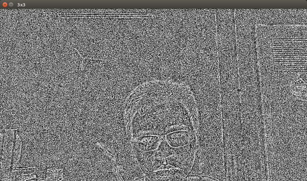
3×3

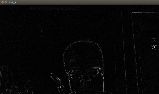
3x3_1

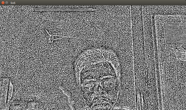
5×5

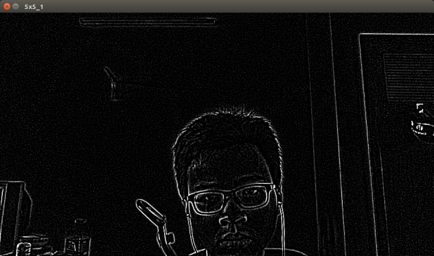
5x5_1

As you can see, the result is very different between cv2.filter2D and scipy.ndarray.convolve.

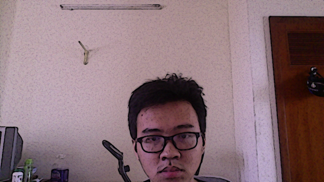
One last example I want to show you is stroking edges in an image. This involve bluring (using cv2.medianFilter), finding edge (using cv2.Laplacian), normalize and inverse image.

import cv2
import numpy as np

def strokeEdge(src, dst, blurKSize = 7, edgeKSize = 5):
    # medianFilter with kernelsize == 7 is expensive
    if blurKSize >= 3:
        # first blur image to cancel noise
        # then convert to grayscale image
        blurredSrc = cv2.medianBlur(src, blurKSize)
        graySrc = cv2.cvtColor(blurredSrc, cv2.COLOR_BGR2GRAY)
    else:
        # scrip blurring image
        graySrc = cv2.cvtColor(src, cv2.COLOR_BGR2GRAY)
    # we have to convert to grayscale since Laplacian only works on grayscale images
    # then we can apply laplacian edge-finding filter
    # cv2.CV_8U means the channel depth is first 8 bits
    cv2.Laplacian(graySrc, cv2.CV_8U, graySrc, ksize=edgeKSize)
    # normalize and inverse color
    # making the edges have black color and background has white color
    normalizedInverseAlpha = (1.0 / 255) * (255 - graySrc)
    channels = cv2.split(src)
    # multiply normalized grayscale image with source image
    # to darken the edge
    for channel in channels:
        channel[:] = channel * normalizedInverseAlpha
    cv2.merge(channels, dst)

Result:

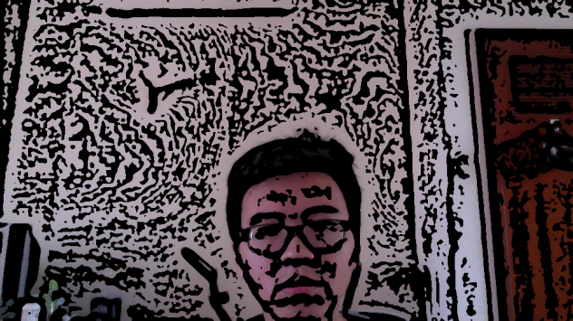
increase ksize of median and Laplacian you will get something like this: